Optimizing trading strategies without overfitting By Ernest Chan and Ray Ng
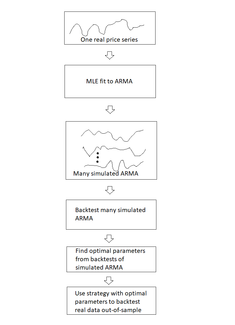
Here is a somewhat trivial example of this procedure. We want to find an optimal strategy that trades AUDCAD on an hourly basis. First, we fit a AR(1)+GARCH(1,1) model to the data using log midprices. The maximum likelihood fit is done using a one-year moving window of historical prices, and the model is refitted every month. We use MATLAB's Econometrics Toolbox for this fit. Once the sequence of monthly models are found, we can use them to predict both the log midprice at the end of the hourly bars, as well as the expected variance of log returns. So a simple trading strategy can be tested: if the expected log return in the next bar is higher than K times the expected volatility (square root of variance) of log returns, buy AUDCAD and hold for one bar, and vice versa for shorts. But what is the optimal K?
Following the procedure outlined above, each time after we fitted a new AR(1)+GARCH(1, 1) model, we use this to simulate the log prices for the next month's worth of hourly bars. In fact, we simulate this 1,000 times, generating 1,000 time series, each with the same number of hourly bars in a month. Then we simply iterate through all reasonable value of K and remember which K generates the highest Sharpe ratio for each simulated time series. We pick the K that most often results in the best Sharpe ratio among the 1,000 simulated time series (i.e. we pick the mode of the distribution of optimal K's across the simulated series). This is the sequence of K's (one for each month) that we use for our final backtest. Below is a sample distribution of optimal K's for a particular month, and the corresponding distribution of Sharpe ratios:
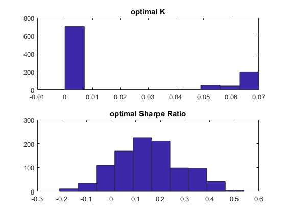 |
| Histogram of optimal K and corresponding Sharpe ratio for 1,000 simulated price series |
Interestingly, the mode of the optimal K is 0 for any month. That certainly makes for a simple trading strategy: just buy whenever the expected log return is positive, and vice versa for shorts. The CAGR is about 4.5% assuming zero transaction costs and midprice executions.
Attachments
No attachments
-
Votes +26
-
Project StrategyQuant X
-
Type Feature
-
Status Archived
-
Priority Normal
-
Assignee Mark Fric
-
Milestone Archived (To be done later)
History
IH
IH
IH
mp
MF
Mark Fric
07.01.2019 11:13Assignee changed from Mark Fric to Mark Fric
Milestone changed from None to Build 118
N
IH
clonex / Ivan Hudec
07.01.2019 19:06
Wow your openness to adding new features like this magnificent. Satisfied that I 2014 I decided to invest do SQ instead of other platforms. You guys doing a spectacular job.
k
DR
a
FB
o
m
l
KW
m
b
KL
KL
kainc301
20.01.2019 10:58
I like this idea but I see there's a heavy reliance on time-based bars. Is there any way to calculate this with non-time-based bars like renkos if this is implemented?
AF
MF
HH
MF
BS
KL
kainc301
30.03.2019 14:12If any more context is needed on this, Ernest Chan goes into detail about this approach here
https://www.youtube.com/watch?v=UD92QBqA8Eo
i
Ad
MF
MF
PS
MF
AA
AA
a
MF
AG
MF
w
A
Votes: +26
© Copyright. All rights reserved. ProjectPanel.com
